Predicting Wine Quality with Deep Learning

 

Deep Learning Problem

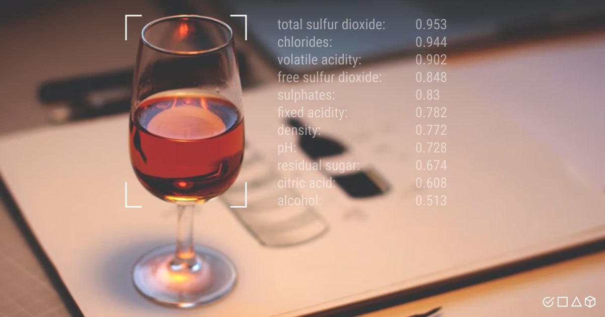
Train the data to check the wine quality

For this purpose we are going to use google colab and in this hands-on practice we will learn each and everything in detail 

Step 1: Problem Statement

We’ll use the Wine Quality Dataset (CSV) to predict wine quality (regression) or classify wine as good/bad (binary classification).

Step 2: Set Up Google Colab

1. Go to Google Colab..

2. Click File → New Notebook.

3. Rename the notebook (e.g., MLP_Wine_Quality_Tutorial or whatever you want).

Step 3: Import Libraries

import numpy as np

import pandas as pd

import matplotlib.pyplot as plt

import seaborn as sns

from sklearn.model_selection import train_test_split

from sklearn.preprocessing import StandardScaler

from sklearn.metrics import accuracy_score, mean_squared_error

import tensorflow as tf

from tensorflow import keras

Now we will see in detail  what these libraries do:                                                                                           

1. Data Handling Libraries

These libraries are useful for managing, analyzing, and manipulating datasets.

numpy (np):

NumPy is used for numerical computations in Python.

It provides powerful array structures and mathematical functions.

Example: It helps in working with arrays and matrices efficiently.

pandas (pd):

Pandas is a data manipulation library that provides DataFrame and Series structures.

It allows for easy reading, writing, and manipulation of structured data.

Example: Reading CSV files, filtering data, handling missing values, etc.

2. Data Visualization Libraries

These libraries help in understanding data distribution and trends.

matplotlib.pyplot (plt):

It is used for creating static, animated, and interactive visualizations.

Example: Drawing line plots, bar charts, scatter plots, etc.

seaborn (sns):

Built on Matplotlib, Seaborn provides enhanced visualization capabilities.

It is useful for drawing more attractive and informative statistical graphs.

Example: Heatmaps, box plots, violin plots, etc.

3. Machine Learning Model Preparation

These libraries help in preprocessing data and splitting it for training and testing.

train_test_split (from sklearn.model_selection):

Splits data into training and testing sets.

Example: 80% training data and 20% testing data.

StandardScaler (from sklearn.preprocessing):

Standardizes features by removing the mean and scaling to unit variance.

Useful when dealing with machine learning models that are sensitive to different data scales.

4. Performance Metrics

These libraries help in evaluating the model's performance.

accuracy_score (from sklearn.metrics):

Measures classification accuracy (used for classification problems).

Example: accuracy_score(y_true, y_pred), where y_true is actual labels and y_pred is predicted labels.

mean_squared_error (from sklearn.metrics):

Measures the difference between predicted and actual values (used for regression problems).

Example: Lower MSE indicates better model performance.

5. Deep Learning Libraries (TensorFlow & Keras)

These libraries are used to build and train deep learning models.

tensorflow (tf):

An open-source library for machine learning and deep learning.

Provides tools for model training and optimization.

keras (from tensorflow):

A high-level neural network API running on top of TensorFlow.

Simplifies the process of building and training deep learning models.

Step 4: Load Data

We’ll use the Wine Quality dataset from Kaggle.

Download the dataset from here (click "Download").

In Colab, click the folder icon (📁) on the left → "Upload" the winequality-red.csv file.

data = pd.read_csv("winequality-red.csv")  # Adjust path if needed

data.head()  # Show first 5 rows

Explore Data

print("Shape:", data.shape)

print("\nMissing values:\n", data.isnull().sum())

print("\nStatistics:\n", data.describe())

Visualize Data

sns.countplot(x="quality", data=data)  # Check class distribution (if classification)

plt.show()

Step 5: Preprocess Data

(1) Define Features (X) and Target (y)

Let’s do binary classification:

Good wine: quality >= 7

Bad wine: quality < 7

data["quality"] = [1 if x >= 7 else 0 for x in data["quality"]]  # Convert to binary

X = data.drop("quality", axis=1)  # Features

y = data["quality"]               # Target

Split Data into Train/Test Sets

X_train, X_test, y_train, y_test = train_test_split(X, y, test_size=0.2, random_state=42)

scaler = StandardScaler()

X_train = scaler.fit_transform(X_train)

X_test = scaler.transform(X_test)

model = keras.Sequential([

    keras.layers.Dense(64, activation="relu", input_shape=(X_train.shape[1],)),  # Hidden layer 1

    keras.layers.Dense(32, activation="relu"),                                   # Hidden layer 2

    keras.layers.Dense(1, activation="sigmoid")                                  # Output layer (binary)

])

model.compile(optimizer="adam", loss="binary_crossentropy", metrics=["accuracy"])

model.summary()  # Check model architecture

for layer in model.layers:

    weights, biases = layer.get_weights()

    print(f"Layer: {layer.name}")

    print(f"Weights Shape: {weights.shape}")

    print(f"Biases Shape: {biases.shape}")

    print("=" * 30)

history = model.fit(

    X_train, y_train,

    epochs=50,

    batch_size=32,

    validation_split=0.2,  # Use 20% of training data for validation

    verbose=1

)

plt.plot(history.history["accuracy"], label="Training Accuracy")

plt.plot(history.history["val_accuracy"], label="Validation Accuracy")

plt.xlabel("Epochs")

plt.ylabel("Accuracy")

plt.legend()

plt.show()

y_pred = (model.predict(X_test) > 0.5).astype("int32")  # Convert probabilities to 0/1

accuracy = accuracy_score(y_test, y_pred)

print(f"Test Accuracy: {accuracy * 100:.2f}%")

from sklearn.metrics import confusion_matrix

cm = confusion_matrix(y_test, y_pred)

sns.heatmap(cm, annot=True, fmt="d")

plt.xlabel("Predicted")

plt.ylabel("True")

plt.show()